Getting started
Installation
Wheels are published for Linux (x86_64, aarch64), macOS (x86_64, Apple
silicon), and Windows. The wheels embed the Rust extension
(gamfit._rust); no Rust toolchain is required at install time.
One-off install without a project:
pip install gamfit also works.
Optional extras
uv add "gamfit[pandas]"     # pandas + pyarrow input/output
uv add "gamfit[plot]"       # matplotlib-based plotting
uv add "gamfit[sklearn]"    # scikit-learn integration
uv add "gamfit[torch]"      # PyTorch bridge
uv add "gamfit[all]"        # everything
gamfit runs without any extra. The extras only affect input/output
conversions and auxiliary modules: without pandas/pyarrow,
predict() returns the format you supplied; without matplotlib,
Model.plot() and posterior trace plots raise; without scikit-learn,
gamfit.sklearn fails to import; without torch, gamfit.torch fails
to import.
Verifying the install
build_info() returns a dict. available: True means the Rust
extension loaded. On available: False, call
gamfit.explain_error(...) for a diagnostic.
First model
import gamfit

train = [
    {"y": 1.2, "x": 0.0},
    {"y": 1.9, "x": 1.0},
    {"y": 3.1, "x": 2.0},
    {"y": 4.5, "x": 3.0},
    {"y": 5.0, "x": 4.0},
]

model = gamfit.fit(train, "y ~ s(x)")
print(model)
gamfit.fit(data, formula) returns a Model. With family="auto" (the
default), the family is inferred from the response column. For a
continuous y this is Gaussian with the identity link. Override with
family= or link=.
s(x) is a cubic P-spline (B-spline basis with a difference penalty).
The basis dimension is chosen from the data unless k= is set. The
smoothing parameter is selected by REML.
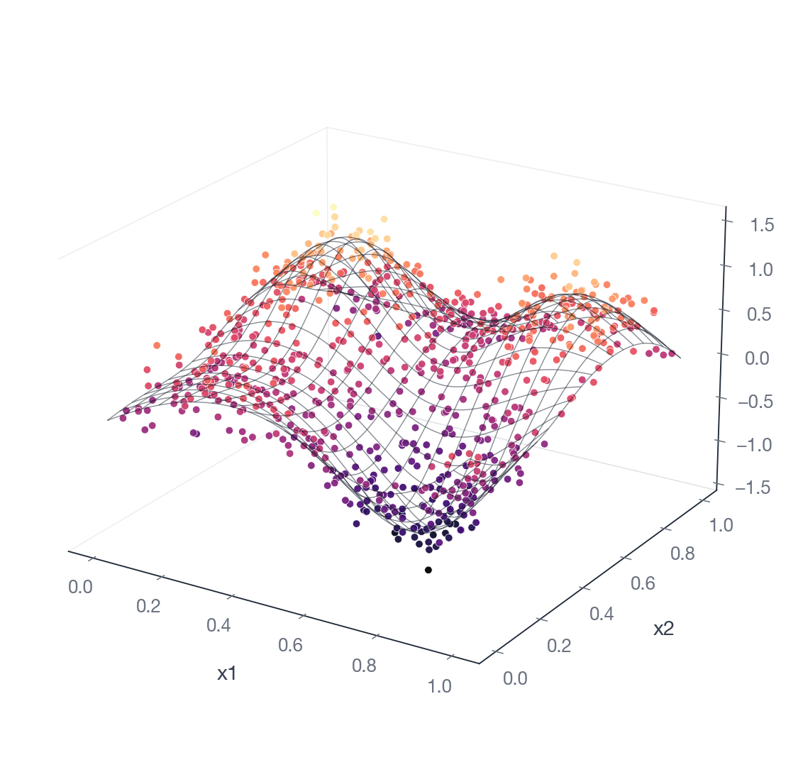
A 2-D smooth fit to scattered observations:
Predict
For Gaussian/binomial/standard models, predict() returns a table with
columns eta (linear predictor) and mean (response-scale). The
container type matches the input or training kind (pandas in, pandas
out, etc.).
For pointwise Wald intervals, pass interval=:
preds = model.predict([{"x": 1.5}, {"x": 2.5}], interval=0.95)
# Columns: eta, mean, effective_se, mean_lower, mean_upper
Transformation-normal and Bernoulli marginal-slope models return a 1-D
NumPy array by default; passing id_column= or return_type= switches
them to the table form. Survival models return a SurvivalPrediction
object with .hazard_at(...), .survival_at(...),
.cumulative_hazard_at(...), and .failure_at(...).
See predictions.md for details on return_type,
id_column, and SurvivalPrediction.
Inspect
model.summary()                     # Summary object
model.diagnose(train).metrics       # n_obs, mae, rmse, bias, r_squared
model.check(test).ok                # schema check against training
model.plot(train, x="x")            # matplotlib (requires gamfit[plot])
model.report("out.html")            # standalone HTML report
Model.summary() returns a Summary carrying the formula, family
name, model class, deviance, REML or LAML score, iteration count, and
per-coefficient estimates with standard errors and credible-interval
bounds. The summary is cached after the first call.
See diagnostics.md for the full list.
Persist
The .gam file is a binary blob; save/load round-trip exactly.
Model.dumps() and gamfit.loads(bytes) are the in-memory equivalents.
See persistence.md.
Posterior sampling
Smoothing parameters are point estimates from REML. To draw from the posterior of the coefficients conditional on those estimates:
posterior = model.sample(train, seed=42)
print(posterior)
# PosteriorSamples(n_draws=..., n_coeffs=8, method='nuts',
#                  rhat=1.004, ess=..., converged=True)

bands = posterior.predict(test, level=0.95)
Defaults for samples, warmup, and chains are derived from the
coefficient count. See posterior-sampling.md
for the exact rule and how to override.
NUTS is used where possible. Gaussian Laplace is the fallback for model classes without an exact NUTS path (location-scale survival, latent survival, location-scale GLMs, transformation-normal, Bernoulli marginal-slope).
Next
- Multiple smooths and constraints: formulas.md.
- Classification, count, positive-continuous data, or non-default links: families-and-links.md.
- Survival data: survival.md; marginal-slope models: marginal-slope.md.
- pandas / pipelines / cross-validation: sklearn.md.
- Worked examples: cookbook.md.