Marginal-slope models

A marginal-slope model fits a standardised risk score z whose effect on the outcome varies across covariate space. The baseline risk surface and the score's log-slope surface live in two separate formulas, so the baseline does not absorb score-specific signal and vice versa.

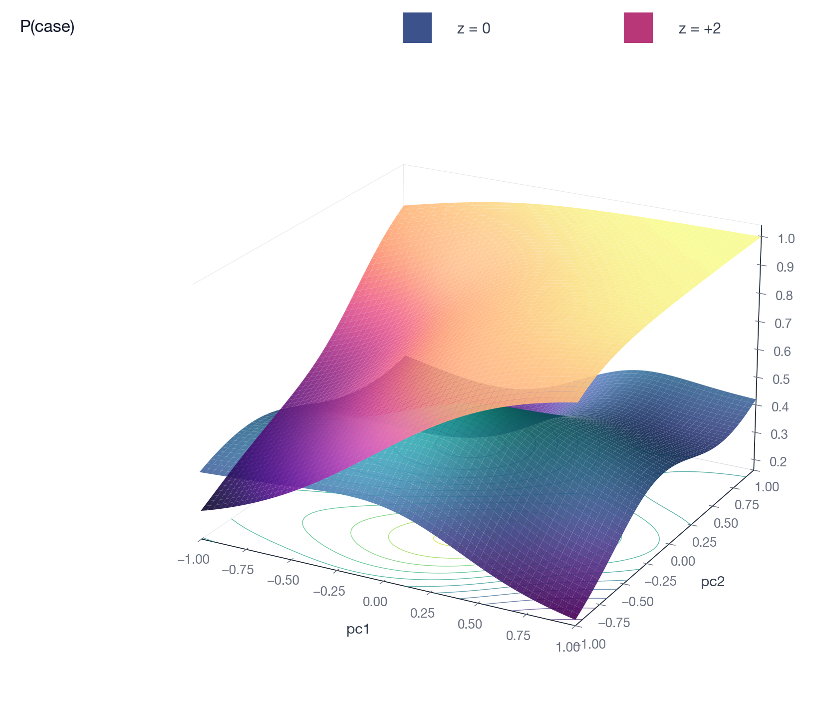
The vertical gap between the two probability surfaces is the risk difference for a unit contrast in z. The modelled score effect lives on the probit/log-slope scale and varies smoothly with covariates.

Two families:

• Bernoulli marginal-slope (family="bernoulli-marginal-slope") for binary outcomes.
• Survival marginal-slope (survival_likelihood="marginal-slope") for time-to-event outcomes.

Both assume z is approximately N(0, 1) conditional on the covariates. Use the transformation-normal calibration step to enforce that.

When to use it

You have:

1. A binary or time-to-event outcome.
2. A continuous risk score that is, or can be made, conditionally N(0, 1).
3. Reason to believe the score's effect size varies across covariates (e.g. across age, ancestry PCs).

A single-coefficient logistic or Cox fit on outcome ~ score + ... forces one slope on the score. Marginal-slope makes the slope itself a smooth function of covariates while leaving the baseline as a separate smooth.

Stage 1: transformation-normal calibration

If the raw score is not already conditionally N(0, 1), fit:

calib = gamfit.fit(
    df,
    "raw_score ~ duchon(pc1, pc2, pc3, pc4, centers=20)",
    transformation_normal=True,
    scale_dimensions=True,
)
df["z"] = calib.predict(df)

transformation_normal=True fits h(score | covariates) ~ N(0, 1). The predict() method of a transformation-normal model returns a 1-D numpy array of z-scores.

Stage 2a: Bernoulli marginal-slope

model = gamfit.fit(
    df,
    "case ~ s(age) + matern(pc1, pc2, pc3)",
    family="bernoulli-marginal-slope",
    link="probit",
    z_column="z",
    logslope_formula="matern(pc1, pc2, pc3)",
    scale_dimensions=True,
)

probs = model.predict(test_df, return_type="dict")["mean"]

• family="bernoulli-marginal-slope" selects the marginal-slope likelihood.
• link="probit": required. The Bernoulli marginal-slope kernel is derived for the probit base link and rejects any other link choice, including flexible(...), blended(...), sas, and beta-logistic.
• z_column="z": name of the conditional z-score column in both the training and prediction tables.
• logslope_formula="...": formula for the log-slope surface as a function of covariates.

The main formula controls the baseline risk; logslope_formula controls the strength of the z effect at each point in covariate space.

CLI equivalent:

gam fit data.csv 'case ~ s(age) + matern(pc1, pc2, pc3)' \
    --logslope-formula 'matern(pc1, pc2, pc3)' --z-column z \
    --scale-dimensions --out model.gam

For vector-valued scores, place the first coordinate in --z-column and add one logslope(z_col, ...) declaration per additional coordinate inside --logslope-formula:

gam fit data.csv 'case ~ s(age) + matern(pc1, pc2, pc3)' \
    --z-column z1 \
    --logslope-formula 'matern(pc1, pc2, pc3) + logslope(z2, s(age)) + logslope(z3, matern(pc1, pc2, pc3))' \
    --scale-dimensions --out model.gam

The unwrapped RHS is the log-slope surface for the first coordinate. Each extra logslope(z_col, ...) adds a surface for that coordinate with its own coefficients and smoothing parameters.

Stage 2b: Survival marginal-slope

model = gamfit.fit(
    df,
    "Surv(entry, exit, event) ~ s(bmi) + s(hba1c)",
    survival_likelihood="marginal-slope",
    z_column="z",
    logslope_formula="s(bmi) + s(hba1c)",
)

pred = model.predict(test_df)
S = pred.survival_at([1, 5, 10])

The main formula specifies the baseline hazard surface; the score's log hazard ratio is a smooth function of covariates given by logslope_formula.

Frailty in marginal-slope survival

Survival marginal-slope supports only frailty_kind="gaussian-shift" with a fixed frailty_sd. "hazard-multiplier" and a learnable gaussian-shift sigma are rejected at fit time.

gamfit.fit(df,
    "Surv(entry, exit, event) ~ s(age)",
    survival_likelihood="marginal-slope",
    z_column="z",
    logslope_formula="s(age)",
    frailty_kind="gaussian-shift",
    frailty_sd=0.3,
)

Detecting marginal-slope models after loading

model = gamfit.load("model.gam")
model.is_marginal_slope            # True if a marginal-slope family
model.is_survival                  # True if survival
model.is_transformation_normal     # True if a Stage 1 calibration model
model.model_class                  # full class string

Notes

• Run Stage 1 (transformation-normal) before Stage 2 so z_column is conditionally N(0, 1).
• Set scale_dimensions=True when calibrating on a handful of PCs so anisotropic length scales are learned per axis.
• Posterior sampling: Bernoulli marginal-slope and transformation-normal models use the Gaussian Laplace approximation in Model.sample(...); survival marginal-slope uses NUTS over the joint coefficient vector. See posterior-sampling.md.
• Predict output: Bernoulli marginal-slope returns a 1-D probability array by default. Pass id_column= or return_type="dict" for a table. The same applies to transformation-normal models.

Two-stage pipeline

import gamfit
import numpy as np
import pandas as pd

n = 1000
rng = np.random.default_rng(0)
df = pd.DataFrame({
    "PGS":  rng.normal(0, 1, n) + 0.3 * rng.normal(0, 1, n),
    "pc1":  rng.normal(0, 1, n),
    "pc2":  rng.normal(0, 1, n),
    "pc3":  rng.normal(0, 1, n),
})
df["disease"] = (rng.uniform(0, 1, n) < 0.25).astype(float)

# Stage 1: condition the score on PCs
calib = gamfit.fit(
    df, "PGS ~ matern(pc1, pc2, pc3, centers=20)",
    transformation_normal=True, scale_dimensions=True,
)
df["pgs_z"] = np.asarray(calib.predict(df), dtype=float)

# Stage 2: Bernoulli marginal-slope
model = gamfit.fit(
    df,
    "disease ~ matern(pc1, pc2, pc3, centers=20)",
    family="bernoulli-marginal-slope",
    link="probit",
    z_column="pgs_z",
    logslope_formula="matern(pc1, pc2, pc3, centers=20)",
    scale_dimensions=True,
)

test = df.head(50).copy()
probs = model.predict(test, return_type="dict")["mean"]